This course enables students to develop an understanding of mathematical concepts related to
algebra, analytic geometry, and measurement and geometry through investigation, the effective
use of technology, and abstract reasoning. Students will investigate relationships, which they
will then generalize as equations of lines, and will determine the connections between different
representations of a linear relation. They will also explore relationships that emerge from the
measurement of three-dimensional figures and two-dimensional shapes. Students will reason
mathematically and communicate their thinking as they solve multi-step problems.
Mathematical process expectations. The mathematical processes are to be integrated into
student learning in all areas of this course.
Throughout this course, students will:
| PROBLEM-SOLVING | � develop, select, apply, and compare a variety of problem-solving strategies as they pose and solve problems and conduct investigations, to help deepen their mathematical understanding; |
| REASONING AND PROVING | � develop and apply reasoning skills (e.g., recognition of relationships, generalization through inductive reasoning, use of counter-examples) to make mathematical conjectures, assess conjectures, and justify conclusions, and plan and construct organized mathematical arguments |
| REFLECTING | � demonstrate that they are reflecting on and monitoring their thinking to help clarify their understanding as they complete an investigation or solve a problem (e.g., by assessing the effectiveness of strategies and processes used, by proposing alternative approaches, by judging the reasonableness of results, by verifying solutions); |
| SELECTING TOOLS AND COMPUTATIONAL STRATEGIES | � select and use a variety of concrete, visual, and electronic learning tools and appropriate computational strategies to investigate mathematical ideas and to solve problems |
| CONNECTING | � make connections among mathematical concepts and procedures, and relate mathematical ideas to situations or phenomena drawn from other contexts (e.g., other curriculum areas, daily life, current events, art and culture, sports); |
| REPRESENTING | � create a variety of representations of mathematical ideas (e.g., numeric, geometric, algebraic, graphical, pictorial representations; onscreen dynamic representations), connect and compare them, and select and apply the appropriate representations to solve problems; |
| COMMUNICATING | � communicate mathematical thinking orally, visually, and in writing, using mathematical vocabulary and a variety of appropriate representations, and observing mathematical conventions |
Number Sense and Algebra
Overall Expectations
By the end of this course, students will:
� demonstrate an understanding of the exponent rules of multiplication and division, and
apply them to simplify expressions;
� manipulate numerical and polynomial expressions, and solve first-degree equations.
Specific Expectations
Operating with Exponents
By the end of this course, students will:
� substitute into and evaluate algebraic expressions involving exponents (i.e., evaluate expressions involving natural-number exponents with rational-number bases [e.g., evaluate (3/2)^3 by hand and 9.83^3 by using a calculator]) (Sample problem: A movie theatre wants to compare the volumes of popcorn in two containers, a cube with edge length 8.1 cm and a cylinder with radius 4.5 cm and height 8.0 cm. Which container holds more popcorn?);
� describe the relationship between the algebraic and geometric representations of a single-variable term up to degree three [i.e., length, which is one dimensional, can be represented by x; area, which is two dimensional, can be represented by (x)(x) or x2; volume, which is three dimensional, can be represented by (x)(x)(x), (x2)(x), or x3];
� derive, through the investigation and examination of patterns, the exponent rules for multiplying and dividing monomials, and apply these rules in expressions involving one and two variables with positive exponents;
� extend the multiplication rule to derive and understand the power of a power rule, and apply it to simplify expressions involving one and two variables with positive exponents.
Manipulating Expressions and Solving Equations
By the end of this course, students will:
� simplify numerical expressions involving integers and rational numbers, with and without the use of technology;*
� solve problems requiring the manipulation of expressions arising from applications of percent, ratio, rate, and proportion;*
� relate their understanding of inverse operations to squaring and taking the square root, and apply inverse operations to simplify expressions and solve equations;
� add and subtract polynomials with up to two variables [e.g., (2x � 5) + (3x + 1), (3x^2y + 2xy^2) + (4x^2y � 6xy^2)], using a variety of tools (e.g., algebra tiles, computer algebra systems, paper and pencil);
� multiply a polynomial by a monomial involving the same variable [e.g., 2x(x + 4), 2x^2(3x^2 � 2x + 1)], using a variety of tools (e.g., algebra tiles, diagrams, computer algebra systems, paper and pencil);
� expand and simplify polynomial expressions involving one variable [e.g., 2x(4x + 1) � 3x(x + 2)], using a variety of tools (e.g., algebra tiles, computer algebra systems, paper and pencil);
� solve first-degree equations, including equations with fractional coefficients, using a variety of tools (e.g., computer algebra systems, paper and pencil) and strategies (e.g., the balance analogy, algebraic strategies);
� rearrange formulas involving variables in the first degree, with and without substitution (e.g., in analytic geometry, in measurement) (Sample problem: A circular garden has a circumference of 30 m. What is the length of a straight path that goes through the centre of this garden?);
� solve problems that can be modeled with first-degree equations, and compare algebraic methods to other solution methods (Sample problem: Solve the following problem in more than one way: Jonah is involved in a walkathon. His goal is to walk 25 km. He begins at 9:00 a.m. and walks at a steady rate of 4 km/h. How many kilometers does he still have left to walk at 1:15 p.m. if he is to achieve his goal?).
*The knowledge and skills described in this expectation are to be introduced as needed and applied and consolidated throughout the course.
Linear Relations
Overall Expectations
By the end of this course, students will:
� apply data-management techniques to investigate relationships between two variables;
� demonstrate an understanding of the characteristics of a linear relation;
� connect various representations of a linear relation.
Specific Expectations
Using Data Management to Investigate Relationships
By the end of this course, students will:
� interpret the meanings of points on scatter plots or graphs that represent linear relations, including scatter plots or graphs in more than one quadrant [e.g., on a scatter plot of height versus age, interpret the point (13, 150) as representing a student who is 13 years old and 150 cm tall; identify points on the graph that represent students who are taller and younger than this student] (Sample problem: Given a graph that represents the relationship of the Celsius scale and the Fahrenheit scale, determine the Celsius equivalent of �5�F.);
� pose problems, identify variables, and formulate hypotheses associated with relationships between two variables (Sample problem: Does the rebound height of a ball depend on the height from which it was dropped?);
� design and carry out an investigation or experiment involving relationships between two variables, including the collection and organization of data, using appropriate methods, equipment, and/or technology (e.g., surveying; using measuring tools, scientific probes, the Internet) and techniques (e.g., making tables, drawing graphs) (Sample problem: Design and perform an experiment to measure and record the temperature of ice water in a plastic cup and ice water in a thermal mug over a 30 min period, for the purpose of comparison. What factors might affect the outcome of this experiment? How could you design the experiment to account for them?);
� describe trends and relationships observed in data, make inferences from data, compare the inferences with hypotheses about the data, and explain any differences between the inferences and the hypotheses (e.g., describe the trend observed in the data. Does a relationship seem to exist? Of what sort? Is the outcome consistent with your hypothesis? Identify and explain any outlying pieces of data. Suggest a formula that relates the variables. How might you vary this experiment to examine other relationships?) (Sample problem: Hypothesize the effect of the length of a pendulum on the time required for the pendulum to make five full swings. Use data to make an inference. Compare the inference with the hypothesis. Are there other relationships you might investigate involving pendulums?).
Understanding Characteristics of Linear Relations
By the end of this course, students will:
� construct tables of values, graphs, and equations, using a variety of tools (e.g., graphing calculators, spreadsheets, graphing software, paper, and pencil), to represent linear relations derived from descriptions of realistic situations (Sample problem: Construct a table of values, a graph, and an equation to represent a monthly cellphone plan that costs $25, plus $0.10 per minute of airtime.);
� construct tables of values, scatter plots, and lines or curves of best fit as appropriate, using a variety of tools (e.g., spreadsheets, graphing software, graphing calculators, paper and pencil), for linearly related and non-linearly related data collected from a variety of sources (e.g., experiments, electronic secondary sources, patterning with concrete materials) (Sample problem: Collect data, using concrete materials or dynamic geometry software, and construct a table of values, a scatter plot, and a line or curve of best fit to represent the following relationships: the volume and the height for a square-based prism with a fixed base; the volume and the side length of the base for a square-based prism with a fixed height.);
� identify, through investigation, some properties of linear relations (i.e., numerically, the first difference is a constant, which represents a constant rate of change; graphically, a straight line represents the relation), and apply these properties to determine whether a relation is linear or non-linear;
� compare the properties of direct variation and partial variation in applications, and identify the initial value (e.g., for a relation described in words, or represented as a graph or an equation) (Sample problem: Yoga costs $20 for registration, plus $8 per class. Tai chi costs $12 per class. Which situation represents a direct variation, and which represents a partial variation? For each relation, what is the initial value? Explain your answers.);
� determine the equation of a line of best fit for a scatter plot, using an informal process (e.g., using a movable line in dynamic statistical software; using a process of trial and error on a graphing calculator; deter mining the equation of the line joining two carefully chosen points on the scatter plot).
Connecting Various Representations of Linear Relations
By the end of this course, students will:
� determine values of a linear relation by using a table of values, by using the equation of the relation, and by interpolating or extrapolating from the graph of the relation (Sample problem: The equation H = 300 � 60t represents the height of a hot air balloon that is initially at 300 m and is descending at a constant rate of 60 m/min. Determine algebraically and graphically how long the balloon will take to reach a height of 160 m.);
� describe a situation that would explain the events illustrated by a given graph of a relationship between two variables (Sample problem: The walk of an individual is illustrated in the given graph, produced by a motion detector and a graphing calculator. Describe the walk [e.g., the initial distance from the motion detector, the rate of walk].);
� determine other representations of a linear relation, given one representation (e.g., given a numeric model, determine a graphical model and an algebraic model; given a graph, determine some points on the graph and determine an algebraic model);
� describe the effects on a linear graph and make the corresponding changes to the linear equation when the conditions of the situation they represent are varied (e.g., given a partial variation graph and an equation representing the cost of producing a yearbook, describe how the graph changes if the cost per book is altered, describe how the graph changes if the fixed costs are altered, and make the corresponding changes to the equation).
Analytic Geometry
Overall Expectations
By the end of this course, students will:
� determine the relationship between the form of an equation and the shape of its graph with
respect to linearity and non-linearity;
� determine, through investigation, the properties of the slope and y-intercept of a linear
relation;
� solve problems involving linear relations.
Specific Expectations
Investigating the Relationship Between the Equation of a Relation and the Shape of Its Graph
By the end of this course, students will:
� determine, through investigation, the characteristics that distinguish the equation of a straight line from the equations of nonlinear relations (e.g., use a graphing calculator or graphing software to graph a variety of linear and non-linear relations from their equations; classify the relations according to the shapes of their graphs; connect an equation of degree one to a linear relation);
� identify, through investigation, the equation of a line in any of the forms y = mx + b, Ax + By + C = 0, x = a, y = b;
� express the equation of a line in the form y = mx + b, given the form Ax + By + C = 0.
Investigating the Properties of Slope
By the end of this course, students will: � determine, through investigation, various formulas for the slope of a line segment or
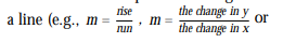
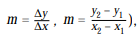
and use the formulas to determine the slope of a line segment or a line;
� identify, through investigation with technology, the geometric significance of m and b in the equation y = mx + b;
� determine, through investigation, connections among the representations of a constant rate of change of a linear relation (e.g., the cost of producing a book of photographs is $50, plus $5 per book, so an equation is C = 50 + 5p; a table of values provides the first difference of 5; the rate of change has a value of 5, which is also the slope of the corresponding line; and 5 is the coefficient of the independent variable, p, in this equation);
� identify, through investigation, properties of the slopes of lines and line segments (e.g., direction, positive or negative rate of change, steepness, parallelism, perpendicularity), using graphing technology to facilitate investigations, where appropriate.
Using the Properties of Linear Relations to Solve Problems
By the end of this course, students will: � graph lines by hand, using a variety of techniques (e.g., graph y = 2x/3 � 4 using the y-intercept and slope; graph 2x + 3y = 6 using the x- and y-intercepts);
� determine the equation of a line from information about the line (e.g., the slope and y-intercept; the slope and a point; two points) (Sample problem: Compare the equations of the lines parallel to and perpendicular to y = 2x � 4, and with the same x-intercept as 3x � 4y = 12.Verify using dynamic geometry software.);
� describe the meaning of the slope and y-intercept for a linear relation arising from a realistic situation (e.g., the cost to rent the community gym is $40 per evening, plus $2 per person for equipment rental; the vertical intercept, 40, represents the $40 cost of renting the gym; the value of the rate of change, 2, represents the $2 cost per person), and describe a situation that could be modeled by a given linear equation (e.g., the linear equation M = 50 + 6d could model the mass of a shipping package, including 50 g for the packaging material, plus 6 g per flyer added to the package);
� identify and explain any restrictions on the variables in a linear relation arising from a realistic situation (e.g., in the relation C = 50 + 25n, C is the cost of holding a party in a hall and n is the number of guests; n is restricted to whole numbers of 100 or less, because of the size of the hall, and C is consequently restricted to $50 to $2550);
� determine graphically the point of intersection of two linear relations, and interpret the intersection point in the context of an application (Sample problem: A video rental company has two monthly plans. Plan A charges a flat fee of $30 for unlimited rentals; Plan B charges $9, plus $3 per video. Use a graphical model to determine the conditions under which you should choose Plan A or Plan B.).
Measurement and Geometry
Overall Expectations
By the end of this course, students will:
� determine, through investigation, the optimal values of various measurements;
� solve problems involving the measurements of two-dimensional shapes and the surface areas
and volumes of three-dimensional figures;
� verify, through investigation facilitated by dynamic geometry software, geometric properties
and relationships involving two-dimensional shapes, and apply the results to solving
problems.
Specific Expectations
Investigating the Optimal Values of Measurements
By the end of this course, students will:
� determine the maximum area of a rectangle with a given perimeter by constructing a variety of rectangles, using a variety of tools (e.g., geoboards, graph paper, toothpicks, a pre-made dynamic geometry sketch), and by examining various values of the area as the side lengths change and the perimeter remains constant;
� determine the minimum perimeter of a rectangle with a given area by constructing a variety of rectangles, using a variety of tools (e.g., geoboards, graph paper, a premade dynamic geometry sketch), and by examining various values of the side lengths and the perimeter as the area stays constant;
� identify, through the investigation with a variety of tools (e.g. concrete materials, computer software), the effect of varying the dimensions on the surface area [or volume] of square-based prisms and cylinders, given a fixed volume [or surface area];
� explain the significance of the optimal area, surface area, or volume in various applications (e.g., the minimum amount of packaging material; the relationship between surface area and heat loss);
� pose and solve problems involving maximization and minimization of measurements of geometric shapes and figures, (e.g., determine the dimensions of the rectangular field with the maximum area that can be enclosed by a fixed amount of fencing, if the fencing is required on only three sides) (Sample problem: Determine the dimensions of a square-based, open-topped prism with a volume of 24 cm^3 and with the minimum surface area.).
Solving Problems Involving Perimeter, Area, Surface Area, and Volume
By the end of this course, students will:
� relate the geometric representation of the Pythagorean theorem and the algebraic representation a^2 + b^2 = c^2;
� solve problems using the Pythagorean theorem, as required in applications (e.g., calculate the height of a cone, given the radius and the slant height, in order to determine the volume of the cone);
� solve problems involving the areas and perimeters of composite two-dimensional shapes (i.e., combinations of rectangles, triangles, parallelograms, trapezoids, and circles) (Sample problem: A new park is in the shape of an isosceles trapezoid with a square attached to the shortest side. The side lengths of the trapezoidal section are 200 m, 500 m, 500 m, and 800 m, and the side length of the square section is 200 m. If the park is to be fully fenced and sodded, how much fencing and sod are required?);
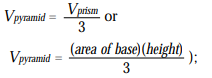
� develop, through investigation (e.g., using concrete materials), the formulas for the volume of a pyramid, a cone, and a sphere (e.g., use three-dimensional figures to show that the volume of a pyramid [or cone] is 2/3 the volume of a prism [or cylinder] with the same base and height, and therefore that
� determine, through investigation, the relationship for calculating the surface area of a pyramid (e.g., use the net of a square based pyramid to determine that the surface area is the area of the square base plus the areas of the four congruent triangles);
� solve problems involving the surface areas and volumes of prisms, pyramids, cylinders, cones, and spheres, including composite figures (Sample problem: Break-bit Cereal is sold in a single-serving size, in a box in the shape of a rectangular prism of dimensions 5 cm by 4 cm by 10 cm. The manufacturer also sells the cereal in a larger size, in a box with dimensions double those of the smaller box. Compare the surface areas and the volumes of the two boxes, and explain the implications of your answers.).
Investigating and Applying Geometric Relationships
By the end of this course, students will:
� determine, through investigation using a variety of tools (e.g., dynamic geometry software, concrete materials), and describe the properties and relationships of the interior and exterior angles of triangles, quadrilaterals, and other polygons, and apply the results to problems involving the angles of polygons (Sample problem: With the assistance of dynamic geometry software, determine the relationship between the sum of the interior angles of a polygon and the number of sides. Use your conclusion to determine the sum of the interior angles of a 20-sided polygon.);
� determine, through investigation using a variety of tools (e.g., dynamic geometry software, paper folding), and describe some properties of polygons (e.g., the figure that results from joining the midpoints of the sides of a quadrilateral is a parallelogram; the diagonals of a rectangle bisect each other; the line segment joining the midpoints of two sides of a triangle is half the length of the third side), and apply the results in problem-solving (e.g., given the width of the base of an A-frame tree house, determine the length of a horizontal support beam that is attached halfway up the sloping sides);
� pose questions about geometric relationships, investigate them, and present their findings, using a variety of mathematical forms (e.g., written explanations, diagrams, dynamic sketches, formulas, tables) (Sample problem: How many diagonals can be drawn from one vertex of a 20-sided polygon? How can I find out without counting them?);
� illustrate a statement about a geometric property by demonstrating the statement with multiple examples, or deny the statement on the basis of a counter-example, with or without the use of dynamic geometry software (Sample problem: Confirm or deny the following statement: If a quadrilateral has perpendicular diagonals, then it is a square.).